Introduction to Data Preprocessing and its Types
Last Updated on by Sarina Sindurakar
What is Data preprocessing?
Data preprocessing is a data mining technique that involves transforming incomplete, inconsistent, and/or noisy data which increase chances of error and misinterpretation, into an understandable format.
- Incomplete: Lacking attribute values, lacking certain attributes of interest, or containing only aggregate data. E.g., occupation = “”
- Noisy: Noisy data is a meaningless data that can’t be interpreted by machines. It can be generated due to faulty data collection, data entry errors etc. E.g., Salary = “-10”
- Inconsistent: Containing discrepancies in codes or names. E.g., Age= “42” Birthday= “03/07/1997”
Data preprocessing is a proven method of resolving issues caused by raw data.
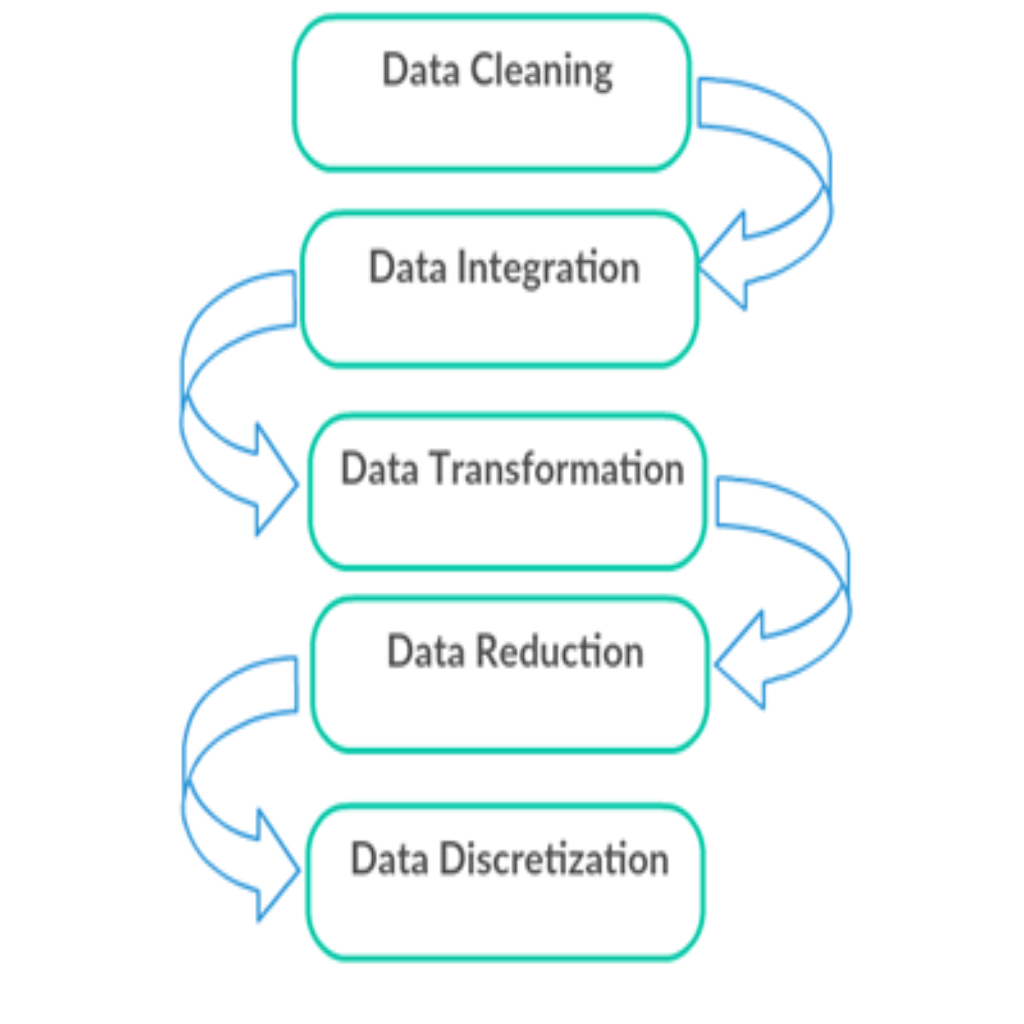
Steps involved in data pre-processing are:
Fig: Data Preprocessing Steps

Data Cleaning
Data cleaning involves handling of missing data, noisy data etc.
a) Missing Data: It can be handled in various ways such as:
- Ignore the tuples: This approach is suitable only when the dataset we have is quite large and multiple values are missing within a tuple.
- Fill in the missing value manually.
- Use a global constant to fill in the missing value. E.g., “unknown”, a new class.
- Use the attribute mean to fill in the missing value.
- Use the attribute mean for all samples belonging to the same class as the given tuple.
- Use the most probable value to fill in the missing value.
b) Noisy Data:
It can be handled in following ways:
- Binning method: To smooth or handle noisy data, firstly, the data is sorted and separated into segments of equal size and stored in the form of bins. There are three methods for smoothing data in the bin.
- Smoothing by bin mean method: In this method, the values in the bin are replaced by the mean value of the bin.
- Smoothing by bin median: In this method, the values in the bin are replaced by the median value.
- Smoothing by bin boundary: In this method, the using minimum and maximum values of the bin values are taken and the values are replaced by the closest boundary value.
- Regression: Here, data can be made smooth by fitting it to a regression function. The regression used may be linear (having one independent variable) or multiple (having multiple independent variables).
- Clustering: This approach groups the similar data in a cluster. The outliers may be undetected or it will fall outside the clusters.
Data Integration
It involves combining data from multiple heterogeneous data sources into a single data store and provide a unified view of the data. These sources may include multiple data cubes, databases, or flat files.
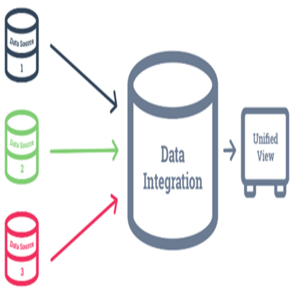

There are mainly 2 major approaches for data integration:
- Tight Coupling: In tight coupling, data is combined from different sources into a single physical location through the process of ETL – Extraction, Transformation and Loading.
- Loose Coupling: In loose coupling, data only remains in the actual source databases. An interface is provided that takes query from user and transforms it in a way the source database can understand and then sends the query directly to the source databases to obtain the result.
Data Transformation
Data transformation is the process of transforming data into the form that is appropriate for mining.
Some Data Transformation Strategies:
- Smoothing: It is used to remove the noise from data. Such techniques include binning, clustering, and regression.
- Aggregation: Here, summary or aggregation operations are applied to the data for analysis of the data at multiple levels.
- Generalization: Here, low-level data are replaced by higher level concepts through the use of concept hierarchies.
- Attribute construction: Here, new attributes are constructed and added from the given set of attributes to help the mining process.
- Normalization: Here the attribute data are scaled so as to fall within a small specified range, such as -1 to +1, or 0 to 1.
Data Reduction
A database or date warehouse may take very long to perform data analysis and mining on huge amounts of data. Data Reduction is a reduced representation of the data set that is much smaller in volume but yet produces the same (or almost the same) analytical results.
Data Reduction Techniques:
- Dimensionality Reduction: Dimensionality reduction is the process of reducing the number of random variables or attributes under consideration. Attribute subset selection is a method of dimensionality reduction in which irrelevant, weakly relevant, or redundant attributes or dimensions are detected and removed. For example,
| Name | Mobile No. | Mobile Network |
| Aarav | 9840xxxxxx | NTC |
| Milan | 9818xxxxxx | NCELL |
If we know Mobile Number, then we can know the Mobile Network. So, we can to reduce that dimension.
| Name | Mobile No. |
| Aarav | 9840xxxxxx |
| Milan | 9818xxxxxx |
- Numerosity Reduction: Numerosity reduction techniques replace the original data volume by alternative, smaller forms of data representation. These techniques may be parametric or nonparametric. For parametric methods, a model is used to estimate the data, so that typically only the data parameters need to be stored, instead of the actual data (Outliers may also be stored.) Regression and log-linear models are examples. Nonparametric methods for storing reduced representations of the data include histograms, clustering, sampling, and data cube aggregation.
- Data Compression: In data compression, transformations are applied so as to obtain a reduced or “compressed” representation of the original data. If the original data can be reconstructed from the compressed data without any information loss, the data reduction is called lossless. If, instead, we can reconstruct only an approximation of the original data, then the data reduction is called lossy.
Data Discretization and Concept Hierarchy
Discretization reduces the number of values for a given continuous attribute by dividing the range of the attribute into intervals. Interval labels can then be used to replace actual data values.
Discretization can be categorized into following two types:
- Top-down discretization: If we first consider one or a couple of points (so-called breakpoints or split points) to divide the whole set of attributes and repeat of this method up to the end, then the process is known as top-down discretization also known as splitting.
- Bottom-up discretization: If we first consider all the constant values as split-points, some are discarded through a combination of the neighborhood values in the interval, that process is called bottom-up discretization.
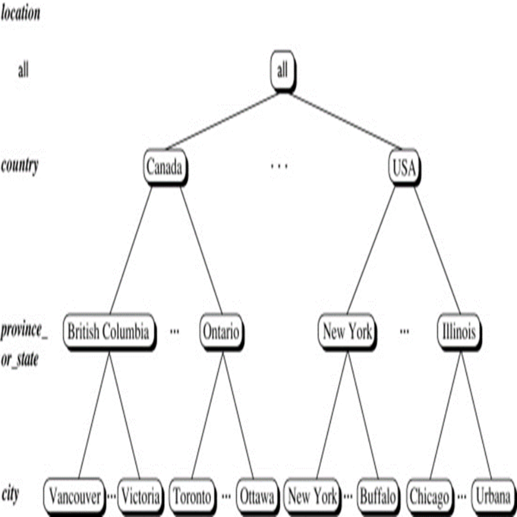
Concept Hierarchies reduce the data by collecting and replacing low level concepts (such as city) by higher level concepts (such as province or country).

Also Read: Why do we need Data mart? Types of Data Mart


